SymPy

So far we have mostly discussed scientific computing from a numerical perspective. Symbolic computing can also done readily in Python using SymPy. The SymPy website has many great tutorials as well as the documentation for SymPy.

An example: Finding wavespeeds of a hyperbolic system

In physics, wavelike phenomena often arise from systems of hyperbolic conservation laws. Generally, these take the form

(1)\[\frac{\partial\textbf{U}}{\partial t} + \nabla\cdot\textbf{F}(\textbf{U}) = 0\]

where \(\textbf{U}\) is a vector of conserved quantities and \(\textbf{F}\) is a flux tensor describing the flow of these quantities. In two space dimensions the above becomes

(2)\[\frac{\partial\textbf{U}}{\partial t} + \frac{\partial\textbf{F}}{\partial x} + \frac{\partial\textbf{G}}{\partial y} = 0\]

where \(\textbf{F} = \left(\textbf{F}(\textbf{U}),\textbf{G}(\textbf{U})\right)\) consists of the \(x\) and \(y\) direction fluxes. We can use the chain rule to decompose the flux derivatives, which gives the so called quasi-linear form of the equation:

(3)\[\frac{\partial\textbf{U}}{\partial t} + \frac{\partial\textbf{F}}{\partial\textbf{U}}\frac{\partial\textbf{U}}{\partial x} + \frac{\partial\textbf{G}}{\partial\textbf{U}}\frac{\partial\textbf{U}}{\partial y} = 0\]

where \(\frac{\partial\textbf{F}}{\partial\textbf{U}}\) and \(\frac{\partial\textbf{G}}{\partial\textbf{U}}\) are Jacobian matrices of each flux. These matrices are interesting both mathematically and physically. In particular, the eigenvalues of these matrices yield the wavespeeds in each direction.

Let’s consider the shallow water equations (in conservation form)

(4)\[\begin{split}\frac{\partial h}{\partial t} &+& \frac{\partial}{\partial x}&(hu) &+& \frac{\partial}{\partial y}(hv) = 0 \\ \frac{\partial (hu)}{\partial t} &+& \frac{\partial}{\partial x}&\left(hu^2 + \frac{1}{2}gh^2\right) &+& \frac{\partial}{\partial y}(huv) = 0 \\ \frac{\partial (hv)}{\partial t} &+& \frac{\partial}{\partial x}&(huv) &+& \frac{\partial}{\partial y}\left(hv^2 + \frac{1}{2}gh^2\right) = 0\end{split}\]

where the conserved variables are the height of the fluid \(h\), and the momenta \(hu\) and \(hv\). Additionally, \(g\) is the gravitational acceleration. The following SymPy code generates the flux Jacobian in the \(x\) direction, and finds the corresponding wavespeeds.

# File: sweEigs.py
# Author: Ian May
# Purpose: Symbolically compute flux Jacobian for 2D shallow
#          water equations and look at eigendecomposition

import sympy as sym

# Shallow water equations depend on:
# h: height, strictly positive
# hu: x-direction momentum
# hv: y-direction momentum
# g: gravitational acc. (constant, positive)
def sweVars():
    h = sym.Symbol('h',positive=True)
    hu = sym.Symbol('hu')
    hv = sym.Symbol('hv')
    g = sym.Symbol('g',positive=True)
    return h,hu,hv,g

# Flux of conserved quantities in x-direction
def fluxX(h,hu,hv,g):
    return sym.Matrix([hu,hu**2/h + g*h**2/2,hu*hv/h])

# Flux of conserved quantities in y-direction
def fluxY(h,hu,hv,g):
    return sym.Matrix([hv,hu*hv/h,hv**2/h + g*h**2/2])

# Jacobian of x-flux wrt. conserved variables
def fluxJacX(h,hu,hv,g):
    return fluxX(h,hu,hv,g).jacobian([h,hu,hv])

# x-direction wavespeeds are e-vals of flux Jacobian
def wavespeedX(h,hu,hv,g):
    return tuple(fluxJacX(h,hu,hv,g).eigenvals().keys())

# Final results can be simplified by using primitive variables
def relations(h,hu,hv,g):
    u = sym.Symbol('u')
    v = sym.Symbol('v')
    rels = {hu/h:u, hv/h:v}
    return rels

if __name__ == '__main__':
    # Setup SWE variables as symbols
    h,hu,hv,g = sweVars()
    # Get wavespeeds as e-vals of flux Jacobian
    wvX = wavespeedX(h,hu,hv,g)
    # Get dictionary of conservative -> primitive vars
    rels = relations(h,hu,hv,g)
    # Try to simplify wavespeeds
    print('Found x-direction wavespeeds as:')
    for w in wvX:
        print(w.subs(rels))
    

Download this code

Exercises:

• Generate \(y\) direction wavespeeds as well

• Generate eigenvectors (waves) of the flux Jacobian

SciPy

SciPy is a Python package that contains numerous scientific toolboxes that are commonly used in the scientific computing community. SciPy is built on top of NumPy, and two work together quite well.

Included in SciPy are implementations of numerical interpolation and quadrature rules, optimization, image processing, statistics, special functions, etc. The routines available in SciPy are highly optimized, robust, and well documented. To see examples of how to use SciPy for scientific computing check out the SciPy users guide

An example: Solving a nonlinear, chaotic, ODE

To demonstrate one small piece of SciPy we’ll solve the Lorenz system of equations:

(5)\[\begin{split}\frac{dx}{dt} &= \sigma (y - x) \\ \frac{dy}{dt} &= x (\rho - z) - y \\ \frac{dz}{dt} &= xy - \beta z\end{split}\]

where \(\rho,\sigma,\beta\) are parameters which we’ll fix at \(28\), \(10\), and \(8/3\) respectively. These equations arise as a highly simplified, reduced order model, for convection as applicable to weather prediction. While quite simple to write down, these equations are nonlinear and can not be solved analytically. Furthermore, they give rise to complex and chaotic behavior, and are arguably the most well known example of a (continuous) chaotic system.

As such, these are a perfect candidate for numerical treatment. SciPy makes solving equations like this nearly trivial, as the following code demonstrates.

# File: lorenz_demo.py
# Author: Ian May
# Purpose: Demonstrate SciPy by solving the Lorenz equations

import numpy as np
import matplotlib.pyplot as plt
from scipy.integrate import solve_ivp

# Define right hand side of ODE
# Note calling signature must look like this
def lorenz(t,y):
    # Parameters for the system
    rho = 28
    sigma = 10
    beta = 8/3
    # Return RHS
    f = np.zeros_like(y)
    f[0] = sigma*(y[1] - y[0])
    f[1] = y[0]*(rho - y[2]) - y[1]
    f[2] = y[0]*y[1] - beta*y[2]
    return f

if __name__ == '__main__':
    # Set initial condition and solve
    t0, tf = 0.0, 100.0
    dt_max = 0.02
    y0 = np.ones(3)
    sol = solve_ivp(lorenz,(t0,tf),y0,max_step=dt_max)

    # Plot time series of each component
    fig, axs = plt.subplots(3,1)

    axs[0].plot(sol.t,sol.y[0,:])
    axs[0].set_ylabel('x',fontsize=14)
    axs[0].set_title('Evolution of Lorenz equations',fontsize=16)
    
    axs[1].plot(sol.t,sol.y[1,:])
    axs[1].set_ylabel('y',fontsize=14)
    
    axs[2].plot(sol.t,sol.y[2,:])
    axs[2].set_xlabel('t',fontsize=14)
    axs[2].set_ylabel('z',fontsize=14)

    fig.tight_layout()
    plt.show()

    # Plot phase space trajectory
    ax = plt.figure().add_subplot(projection='3d')
    
    ax.plot(sol.y[0,:],sol.y[1,:],sol.y[2,:])

    ax.set_xlabel('x',fontsize=15)
    ax.set_ylabel('y',fontsize=15)
    ax.set_zlabel('z',fontsize=15)
    ax.set_title('Lorenz phase space trajectory',fontsize=18)

    plt.show()

Download this code

This should have produced the following two figures.

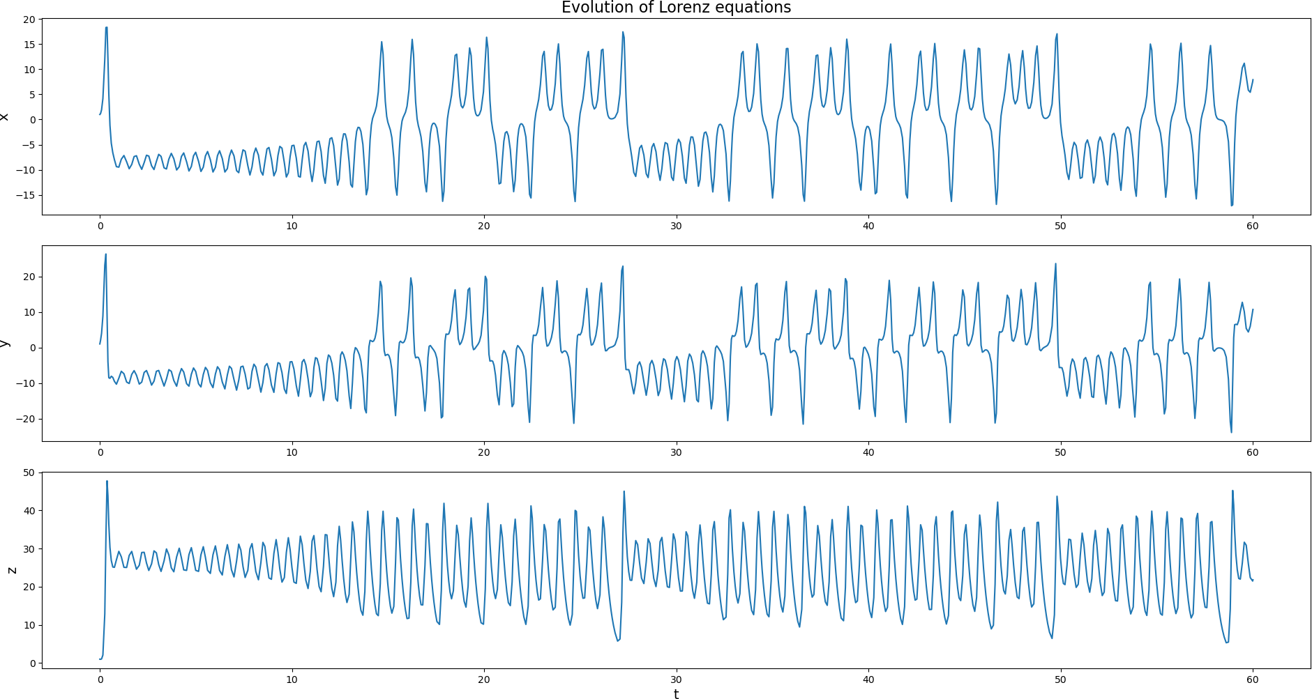
Time history of each component in the Lorenz system

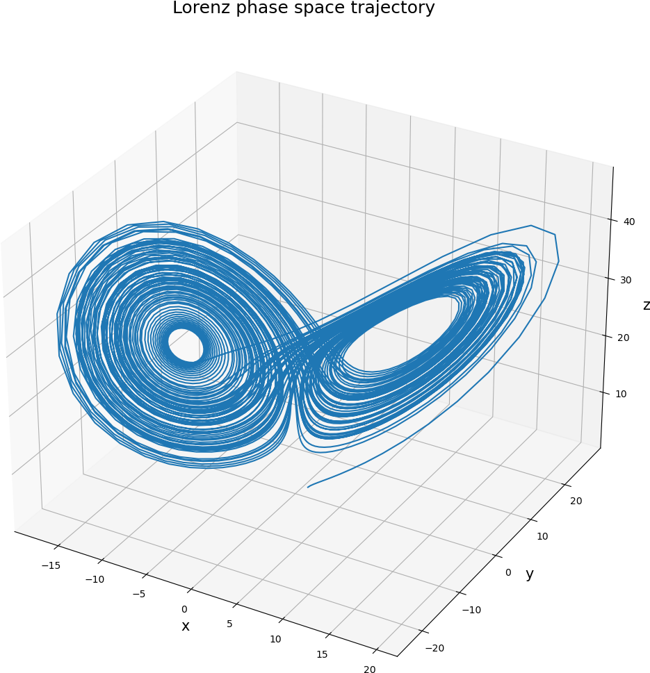
Phase space trajectory of the Lorenz system from the given initial condition.