Outlook

Google drive folder with Jupyter Notebooks used in class: Jupyter Notebooks from class

In this chapter, we are going to learn how to support our endeavors in scientific computing with NumPy, matplotlib, and a few other tools. As we already have seen, NumPy is one of the core mathematical tools for numerical computing in Python. We’ll first cover how to handle mathematical objects using NumPy. Then we’ll look at how to produce nice looking plots using Matplotlib – the core plotting tool for Python.

Following these topics we will also look at symbolic calculation using the SymPy package, more specialized numerical tools in the SciPy package, and then close out with a glance at some higher level libraries that combine many of these tools together.

Reading Materials

The materials of this chapter in part have been adopted and modified from:

• SciPy Lecture Notes,

• Prof. LeVeque’s (Univ. of Washington) online note on Python.

Array manipulations in NumPy

Arrays are an essential construct in scientific computing. For example, an array can contain:

• 2D fields or images recorded through experiment or simulation

• Solutions of PDE on logically rectangular grids in 2, 3, or more dimensions

• Time varying signals recorded by one or more measurement devices

• and many, many more

Wait a minute… we already have something like this, i.e., Python lists! Unfortunately, Python lists are not suitable for numerical computing. First, let’s see why.

Python lists vs. NumPy arrays

Python has lists as a built-in data type, e.g.

>>> x = [1., 2., 3.]

defines a list that contains 3 real numbers and might be viewed as a vector. However, you cannot easily do arithmetic on such lists the way we could in Fortran, e.g. 2*x does not give [2., 4., 6.] as you might hope. Trying this produces:

>>> 2*x
[1.0, 2.0, 3.0, 1.0, 2.0, 3.0]

Instead of doubling the elements of the list this doubles the length of x by appending another copy (x + x would give the same thing). These are certainly not the results of scaling or adding vectors.

Two-dimensional arrays are also a bit clumsy when using Python lists, as they have to be specified as a list of lists, e.g., a \(3\times 2\) array with the elements 11,12 in the first row, 21,22 in the second row, 31,32 in the third row would be specified by

>>> A = [[11, 12], [21, 22], [31, 32]]

Note that indexing always starts with 0 in Python, so we find for example that

>>> A[0]
[11, 12]
>>> A[1]
[21, 22]
>>> A[1][0]
21

Here A[0] refers to the 0-index element of A, which is itself a list [11, 12]. A[1][0] can be understood as the 0-index element of A[1] = [21, 22], hence A[1][0] is 21.

Working with A as a matrix would be quite clumsy. Any non-trivial operation would require explicit loops over the entries. Most importantly, these loops would have to be done inside Python.

NumPy was developed to make it easy to do the sorts of things we want to do with matrices and vectors, and more generally n-dimensional arrays. Importantly, most operations on NumPy arrays call out to highly optimized precompiled code. This means that any required looping happens outside of Python.

For example

>>> import numpy as np
>>> x = np.array([1., 2., 3.])
>>> x
array([ 1.,  2.,  3.])

>>> 2*x
array([ 2.,  4.,  6.])

>>> np.sqrt(x)
array([ 1.        ,  1.41421356,  1.73205081])

We see that we can multiply by a scalar or take component-wise square roots. Indeed, the syntax is very reminiscent of Fortran. We can slice arrays, broadcast products, and do elementwise operations easily.

Performance comparison

NumPy arrays are more efficient than Python lists, particularly when applying a mathematical operation to the whole array.

To see the different behavior, we can use the timeit module which gives a simple way to time small bits of Python code. For a more full description, see the documentation.

For instance, timing an operation on a regular Python’s list

>>> import timeit
>>> tList = timeit.Timer('[i**2 for i in L]',setup='L=range(50)')
>>> tList.timeit()
7.368645437993109

On the contrary, timing an operation on a NumPy array of the same size gives:

>>> import timeit  # not needed if imported already
>>> setupArr = '''
... import numpy as np
... a = np.arange(50)
... '''
>>> tArr = timeit.Timer('a**2',setup=setupArr)
>>> tArr.timeit()
0.6314092200191226

which is substantially faster, and even includes the time required to import numpy.

Creating NumPy data arrays

We looked at a brief example of initializing a NumPy array in the above, where individual items were given explicitly as inputs. In practice, however, we probably want to avoid adding items one by one. Some common examples are as follows:

• Evenly spaced values (best for integers)

  >>> import numpy as np
  >>> a = np.arange(10) # np.arange(n) provides indices from 0 to n-1
  >>> a
  array([0, 1, 2, 3, 4, 5, 6, 7, 8, 9])
  >>> a.dtype
  dtype('int64')
  >>> b = np.arange(1., 9., 2) # syntax : start, end, step
  >>> b
  array([ 1.,  3.,  5.,  7.])
  >>> b.dtype
  dtype('float64')
  

  or by specifying the number of points (best for floats)

  >>> c = np.linspace(0, 1, 6)
  >>> c
  array([ 0. ,  0.2,  0.4,  0.6,  0.8,  1. ])
  >>> d = np.linspace(0, 1, 5, endpoint=False)
  >>> d
  array([ 0. ,  0.2,  0.4,  0.6,  0.8])
  

  Alternatively, you can use np.arange to get floats by specifying the data type:

  >>> a = np.arange(10, dtype=np.float64)
  

• There are built-in constructors for several of the most common arrays. These include arrays of all ones, all zeros, identity arrays, and diagonal arrays (among others).

  >>> a = np.ones((3,3))
  >>> a
  array([[ 1.,  1.,  1.],
         [ 1.,  1.,  1.],
         [ 1.,  1.,  1.]])
  >>> a.dtype
  dtype('float64')
  >>> b = np.ones(5, dtype=np.int)
  >>> b
  array([1, 1, 1, 1, 1])
  >>> c = np.zeros((2,3))
  >>> c
  array([[ 0., 0., 0.],
         [ 0., 0., 0.]])
  >>> d = np.eye(3)
  >>> d
  array([[ 1.,  0.,  0.],
         [ 0.,  1.,  0.],
         [ 0.,  0.,  1.]])
  

  The first argument in each case is a tuple with the size of each dimension in the desired array. Compare this to the dimension(M,N,...) keyword in Fortran.

Note

Just like Fortran arrays have a maximum rank (compiler dependent), NumPy arrays have a maximum rank. Currently this cap is 32. If you’re problem requires more than 32 dimensions, you should strongly consider finding an alternative way to pose the problem. For more information, try reading up on the curse of dimensionality.

• You can also create arrays using nested python lists, which is good for entering small arrays by hand. The \(3\times 2\) array from above could be written as

  A = np.array([[11, 12], [21, 22], [31, 32]])
  

Querying properties of NumPy arrays

In Fortran we used the size intrinsic function to write functions and subroutines that worked for any size array as long as the rank was known. NumPy arrays support similar queries. A few quite useful ones are:

• Get the data type of the elements

  >>> print(A.dtype)
  int64
  

  Note that this is not necessarily the same as Python’s intrinsic int type. Similarly, floats will default to

  >>> B = np.array([1.0,2.0])
  >>> print(B.dtype)
  float64
  

  Often these are the same as the Python intrinsics, but NumPy is capable of storing many different types. See more here.

• Get the number of dimensions (rank)

  >>> print(A.ndim)
  2
  

• Get the shape of the array

  >>> s = A.shape
  >>> print(s)
  (3, 2)
  >>> print(type(s))
  <class 'tuple'>
  

• Get the size of the array

  >>> s = A.size
  >>> print(s)
  6
  >>> print(type(s))
  <class 'int'>
  

  Note that size is the total number of elements, while shape is the number of elements along each rank of the array.

NumPy array indexing

The items of an array can be accessed in a similar same way to the other Python sequences (list, tuple)

>>> a = np.arange(10)
>>> a
array([0, 1, 2, 3, 4, 5, 6, 7, 8, 9])
>>> b = a[0], a[2], a[-1]
>>> b
(0, 2, 9)
>>> type(b)
tuple

For a multidimensional array a, indexes are tuples of integers, that is, for a 3D array, a[(i,j,k)], or simply a[i,j,k]

 >>> a = np.diag(np.arange(5))
 >>> a
 array([[0, 0, 0, 0, 0],
        [0, 1, 0, 0, 0],
        [0, 0, 2, 0, 0],
        [0, 0, 0, 3, 0],
        [0, 0, 0, 0, 4]])
>>> a[1,1]
1
>>> a[2,1] = 10 # third line (or row), second column
>>> a
array([[ 0,  0,  0,  0,  0],
       [ 0,  1,  0,  0,  0],
       [ 0, 10,  2,  0,  0],
       [ 0,  0,  0,  3,  0],
       [ 0,  0,  0,  0,  4]])
>>> a[2]   # this is the same as a[2,:]
array([ 0, 10,  2,  0,  0])

Note that:

• All indices occur in one pair of square brackets

• In 2D, the first dimension corresponds to lines (i.e., rows), the second to columns.

• For an array a with more than one dimension, a[i] is interpreted as a[i,:] or a[i,:,:] (or whatever rank is needed).

NumPy array slicing and masking

Slicing extracts multiple elements out of an array simultaneously, and works in a comparable way to list indexing:

>>> a = np.arange(10)
>>> a
array([0, 1, 2, 3, 4, 5, 6, 7, 8, 9])
>>> a[2:8:2] # [start:end:step]
array([2, 4, 6])

Note that the last index is not included!

>>> a[:4]
array([0, 1, 2, 3])

start:end:step is a slice object which represents the set of indices range(start, end, step). Slice objects can also be created explicitly:

>>> sl = slice(1, 9, 2)
>>> a = np.arange(10)
>>> b = 2*a + 1
>>> a, b
(array([0, 1, 2, 3, 4, 5, 6, 7, 8, 9]), array([ 1,  3,  5,  7,  9, 11, 13, 15, 17, 19]))
>>> a[sl], b[sl]
(array([1, 3, 5, 7]), array([ 3,  7, 11, 15]))

All three slice components are not required: by default, start is 0, end is the last index in the associated rank, and step is 1. Using these defaults we can do all of the following:

>>> a[1:3]
array([1, 2])
>>> a[::2]
array([0, 2, 4, 6, 8])
>>> a[3:]
array([3, 4, 5, 6, 7, 8, 9])

Question: What is the difference between a[0:2] and a[0::2]?

Of course, all of this works with multidimensional arrays too:

>>> a = np.eye(5)
>>> a
array([[ 1.,  0.,  0.,  0.,  0.],
       [ 0.,  1.,  0.,  0.,  0.],
       [ 0.,  0.,  1.,  0.,  0.],
       [ 0.,  0.,  0.,  1.,  0.],
       [ 0.,  0.,  0.,  0.,  1.]])
>>> a[2:4,:3] #3rd and 4th rows, 3 first columns
array([[ 0.,  0.,  1.],
       [ 0.,  0.,  0.]])

All elements specified by a slice can be easily modified

>>> a[:3,:3] = 4
>>> a
array([[ 4.,  4.,  4.,  0.,  0.],
       [ 4.,  4.,  4.,  0.,  0.],
       [ 4.,  4.,  4.,  0.,  0.],
       [ 0.,  0.,  0.,  1.,  0.],
       [ 0.,  0.,  0.,  0.,  1.]])

Here is a small illustrated summary of NumPy indexing and slicing:

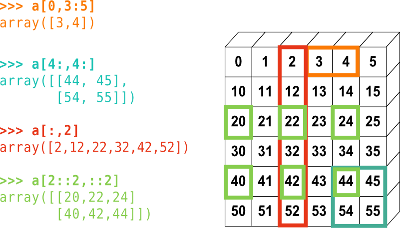
NumPy array indexing.

You can also combine assignment and slicing

>>> a = np.arange(10)
>>> a[5:] = 10
>>> a
array([ 0,  1,  2,  3,  4, 10, 10, 10, 10, 10])
>>> b = np.arange(5)
>>> a[5:] = b[::-1]
>>> a
array([0, 1, 2, 3, 4, 4, 3, 2, 1, 0])

We can also mask parts of the array using a boolean array in place of the slice object. For instance:

>>> B = np.eye(5)
>>> B
array([[1., 0., 0., 0., 0.],
       [0., 1., 0., 0., 0.],
       [0., 0., 1., 0., 0.],
       [0., 0., 0., 1., 0.],
       [0., 0., 0., 0., 1.]])
>>> mask = B<0.5
>>> mask
array([[False,  True,  True,  True,  True],
       [ True, False,  True,  True,  True],
       [ True,  True, False,  True,  True],
       [ True,  True,  True, False,  True],
       [ True,  True,  True,  True, False]])
>>> B[mask] = -2.0
>>> B
array([[ 1., -2., -2., -2., -2.],
       [-2.,  1., -2., -2., -2.],
       [-2., -2.,  1., -2., -2.],
       [-2., -2., -2.,  1., -2.],
       [-2., -2., -2., -2.,  1.]])

You can also create the mask in place. The assignment ``B[mask] = -2.0``
could have instead been written as ``B[B<0.5] = -2.0``.

Copies and views

A slicing operation creates a view of the original array, which is just a way of accessing array data. Thus the original array is not copied in memory. You can use np.may_share_memory() to check if two arrays share the same memory block. Note, however, that this uses heuristics and may give you false positives. It may seem a little odd that this isn’t a guaranteed answer. We’ll return to why this is when we talk about C and pointer aliasing.

When modifying the view, the original array is modified as well

>>> a = np.arange(10)
>>> a
array([0, 1, 2, 3, 4, 5, 6, 7, 8, 9])
>>> b = a[::2]
>>> b
array([0, 2, 4, 6, 8])
>>> np.may_share_memory(a, b)
True
>>> b[0] = 12
>>> b
array([12,  2,  4,  6,  8])
>>> a   # (!)
array([12,  1,  2,  3,  4,  5,  6,  7,  8,  9])

>>> c = a[::2].copy()  # force a copy
>>> c[0] = 47
>>> a
array([12, 1, 2, 3, 4, 5, 6, 7, 8, 9])
>>> c
array([47,  2,  4,  6,  8])

>>> np.may_share_memory(a, c)
False

Note

You can not create a view using an implicit mask, e.g. b = a[a<3] will create a distinct copy. Additionally, this will always return a rank 1 array regardless of the shape of the original array.

Linear algebraic operations

NumPy arrays behave a lot like Fortran arrays under arithmetic. Most operations will default to being performed elementwise. If you are accustomed to MatLab, you should be careful. Here A*B will be an elementwise product, and not a matrix-matrix product (the MatLab equivalent would be A.*B). To get a matrix-matrix product you must use dot, matmul or the @ operator

>>> A = np.array([[1,2], [3,4]])
>>> B = np.array([[5,0], [0,7]])
>>> A
array([[1, 2],
       [3, 4]])
>>> B
array([[5, 0],
       [0, 7]])
>>> A*B            # this will not give a matrix-product, but an elementwise product
array([[ 5,  0],
       [ 0, 28]])
>>> np.dot(A,B)    # this is the expected matrix multiplication
array([[ 5, 14],
       [15, 28]])
>>> B.dot(A)       # Matrix multiplication is not commutative!
array([[ 5, 10],
       [21, 28]])
>>> np.matmul(A,B) # Note: matmul is not a member function of ndarray
...
>>> B @ A
...

Note

The np.dot function generalizes to higher rank tensors. However, that generality comes with a performance penalty. You should use np.matmul or the @ operator whenever possible. It also makes the code a bit easier to read, though that is subjective.

Consult also the functions np.tensordot and np.vdot for other use cases.

Many other linear algebra tools can be found in NumPy. For example, to solve a linear system Ax = b using Gaussian Elimination, we can do

>>> A
array([[1, 2],
       [3, 4]])

>>> b = np.array([2,3])
>>> x = np.linalg.solve(A,b)

>>> x
array([-1. ,  1.5])

To find the eigenvalues and eigenvectors of A we can do:

>>> evals, evecs = np.linalg.eig(A)

>>> evals
array([-0.37228132,  5.37228132])

>>> evecs
array([[-0.82456484, -0.41597356],
       [ 0.56576746, -0.90937671]])

Note

You may be tempted to use the variable name lambda for the eigenvalues of a matrix, but this isn’t allowed in Python because lambda is a keyword of the language.

Reductions of NumPy arrays

In this context, reductions are operations that map arrays to individual scalar values or arrays of lower rank. These include operations like summation, norms, max/min values, etc.

To compute sums

>>> x = np.array([1, 2, 3, 4])
>>> np.sum(x)
10
>>> x.sum()
10

Sum by rows and by columns

>>> x = np.array([[1, 2], [3, 4]])
>>> x
array([[1, 2],
       [3, 4]])
>>> x.sum(axis=0)   # sum along columns (first dimension)
array([4, 6])
>>> x[:, 0].sum(), x[:, 1].sum()
(4, 6)
>>> x.sum(axis=1)   # sum along rows (second dimension)
array([3, 7])
>>> x[0, :].sum(), x[1, :].sum()
(3, 7)

or similarly in even higher dimensions

>>> x = np.array([ [[1,6],[7,4]], [[5,2],[3,8]] ] )
>>> x
array([[[1, 6],
        [7, 4]],

       [[5, 2],
        [3, 8]]])
>>> x.sum(axis = 0)
array([[ 6,  8],
       [10, 12]])
>>> x.sum(axis = 1)
array([[8, 10],
       [8, 10]])
>>> x.sum(axis = 2)
array([[7, 11],
       [7, 11]])

To obtain extrema

>>> x.min()
1
>>> x.max()
8
>>> x.max(axis=0)
array([[5, 6],
       [7, 8]])
>>> x.argmin()  # index of minimum in flattened array
0
>>> x.argmax(axis=0)  # index of maxima along 0th dimension
array([[1, 0],
       [0, 1]])

Logical operations

>>> np.all([True, True, False])
False
>>> np.any([True, True, False])
True
>>> np.all(x<3)
False
>>> np.any(x<3)
True

Finally, we can list a few examples from statistics

>>> x = np.array([1, 2, 3, 1])
>>> y = np.array([[1, 2, 3], [5, 6, 1]])
>>> x.mean()
1.75
>>> np.median(x)
1.5
>>> np.median(y, axis=-1) # last axis, equivalently, np.median(y, axis=1)
array([ 2.,  5.])

>>> x.std()          # full population standard deviation.
0.82915619758884995

Loading data files

Text files

Consider an example: populations.txt:

# year	hare	lynx	carrot
1900	30e3	4e3	48300
1901	47.2e3	6.1e3	48200
1902	70.2e3	9.8e3	41500
1903	77.4e3	35.2e3	38200
1904	36.3e3	59.4e3	40600
1905	20.6e3	41.7e3	39800
1906	18.1e3	19e3	38600
1907	21.4e3	13e3	42300
1908	22e3	8.3e3	44500
1909	25.4e3	9.1e3	42100
1910	27.1e3	7.4e3	46000
1911	40.3e3	8e3	46800
1912	57e3	12.3e3	43800
1913	76.6e3	19.5e3	40900
1914	52.3e3	45.7e3	39400
1915	19.5e3	51.1e3	39000
1916	11.2e3	29.7e3	36700
1917	7.6e3	15.8e3	41800
1918	14.6e3	9.7e3	43300
1919	16.2e3	10.1e3	41300
1920	24.7e3	8.6e3	47300

Download this data

To load populations.txt

 >>> data = np.loadtxt('populations.txt')
 >>> data
 array([[  1900.,  30000.,   4000.,  48300.],
        [  1901.,  47200.,   6100.,  48200.],
        [  1902.,  70200.,   9800.,  41500.],
...
>>> np.mean(data[:,1:],axis=0)
array([34080.95238095, 20166.66666667, 42400.        ])
>>> np.std(data[:,1:],axis=0)
array([20897.90645809, 16254.59153691,  3322.50622558])

To save it to another name, pop2.txt

>>> np.savetxt('pop2.txt', data)

Other well-known file formats

• HDF5: h5py, PyTables

  • We will look at some examples regarding reading in HDF5 files after we cover matplotlib

• NetCDF: scipy.io.netcdf_file, netcdf4-python, others

• Matlab: scipy.io.loadmat, scipy.io.savemat

• IDL: scipy.io.readsav

An example: Numerical differentiation

Differential equations and dynamical systems are ubiquitous in science, and by extension, in scientific computing. One will often need to approximate the derivative of a function knowing only its values at discrete points.

One particularly simple way to approximate derivatives is through finite differences. These get their name from revisiting the limit definition of a derivative

(1)\[\frac{df}{dx} := \lim\limits_{h\rightarrow 0} \frac{f(x+h) - f(x)}{h}\]

and taking \(h\) to be a finite instead of infinitesimal value. This same idea can be extended to higher derivatives and more accurate approximations. Some of the final projects will dig into these methods more deeply.

In this example we’ll use NumPy to approximate the first and second derivative of a function on a uniform grid.

# File: finiteDiff.py
# Author: Ian May
# Purpose: Demonstrate numpy array functionality by
#          computing a few finite differences

import numpy as np
import matplotlib.pyplot as plt

# First derivative using forward difference
def fwdFirstDiff(f,x):
    dx = x[1] - x[0]
    df = (f[1:] - f[:-1])/dx
    return df,x[:-1]

# First derivative using centered difference
def ctrFirstDiff(f,x):
    dx = x[1] - x[0]
    df = (f[2:] - f[:-2])/(2.0*dx)
    return df,x[1:-1]

# Second derivative using centered difference
def ctrSecondDiff(f,x):
    dx = x[1] - x[0]
    ddf = (f[2:] - 2.0*f[1:-1] + f[:-2])/dx**2
    return ddf,x[1:-1]

# Function to approximate and its exact derivatives
def fun(x):
    return np.sin(x**2)

def exactFirstDiff(x):
    return 2.0*x*np.cos(x**2)

def exactSecondDiff(x):
    return 2.0*(np.cos(x**2) - 2.0*x**2*np.sin(x**2))

if __name__=="__main__":
    # Grid and discrete function
    N = 200
    x = np.linspace(0,np.pi,N)
    f = fun(x)
    # Forward first difference
    fFD,xf = fwdFirstDiff(f,x)
    # centered first difference
    cFD,xc = ctrFirstDiff(f,x)
    # centered second difference
    cSD,xc = ctrSecondDiff(f,x)
    # Evaluate error using known exact derivatives
    ex_fFD = exactFirstDiff(xf)
    ex_cFD = exactFirstDiff(xc)
    ex_cSD = exactSecondDiff(xc)
    print('Max error fwd first diff:',np.max(np.abs(fFD - ex_fFD)))
    print('Max error ctr first diff:',np.max(np.abs(cFD - ex_cFD)))
    print('Max error ctr second diff:',np.max(np.abs(cSD - ex_cSD)))

Download this code

Exercises:

• Modify the code to report the relative error instead of absolute error

• Modify the code to report the space-averaged error instead of pointwise error - E.g. report the \(L_1\) error instead of the \(L_\infty\) error

An example: Revisiting HW3

Here we’ll look at an example program using NumPy that solves the same boundary value problem as in the second homework. The initial code is:

# File: dftBvp.py
# Author: Ian May
# Purpose: Define a brief spectral collocation method for the
#          shifted Poisson equation. Written primarily to
#          showcase basic numpy usage

import numpy as np

# Define spatial grid
def grid(N):
    return np.linspace(0,2*np.pi,N,endpoint=False)

# Define wavenumbers and forward transform
def transMat(x):
    N = len(x)
    dx = x[1]-x[0]
    om = 2*np.pi/(N*dx)
    # Set wavenumbers and transformation matrix
    k = np.zeros(N)
    T = np.zeros([N,N])
    T[0,:] = 1./N
    for i in np.arange(1,N,2):
        k[i] = (i+1)*om/2
        T[i,:] = 2*np.cos(k[i]*x)/N
        if(i+1<N):
            k[i+1] = k[i]
            T[i+1,:] = 2*np.sin(k[i]*x)/N
    if(N%2==0):
        T[N-1,:] /= 2
    return (k,T)

# Define inverse transformation
def invTransMat(x,k):
    N = len(x)
    Tinv = np.zeros([N,N])
    Tinv[:,0] = 1.
    for j in np.arange(1,N,2):
        Tinv[:,j] = np.cos(k[j]*x)
    for j in np.arange(2,N,2):
        Tinv[:,j] = np.sin(k[j]*x)
    return Tinv

# Define forcing function and exact solution
def forcing(x):
    es = np.exp(np.sin(x))*(1+np.sin(x)-np.cos(x)**2)
    ec = 9*np.exp(np.cos(3*x))*(-1./9.+np.sin(3*x)**2-np.cos(3*x))
    return es+ec

def exact(x):
    return np.exp(np.sin(x))-np.exp(np.cos(3*x))

# Define default behavior when calling from the command line
if __name__ == "__main__":
    N = 21
    print("Solving with %d grid points" % N)
    # We should wrap this into its own function shouldn't we?
    x = grid(N)
    k,T = transMat(x)
    Tinv = invTransMat(x,k)
    f = forcing(x)
    ft = np.matmul(T,f)
    ft = ft/(1+k**2)
    u = np.matmul(Tinv,ft)
    print("Max error: ", np.max(np.abs(u-exact(x))))

Download this code

First, we can run this directly from the command line to get the same answer as what we saw in the homework for \(N=21\):

$ python dftBvp.py
$ Solving with 21 grid points
$ Max error:  0.009817949242564072

As an exercise, let’s now consider the following:

1. Add a function to wrap the steps required to go from a forcing function to a solution.

2. Loop over a variety of resolutions and record the maximum errors we obtain.

3. Segue into the next section by plotting the solution and forcing function.

An example: Spectra of random matrices

There are some fascinating results regarding the spectra of (large) random symmetric matrices. The study of these spectra first arose in nuclear physics, but have since seen applications in number theory, theoretical neuroscience, and optimal control. The wiki page on Random Matrices has plenty more information.

Let’s consider this problem numerically instead of analytically. We are going to generate a large number of random symmetric \(N\times N\) matrices \(\mathbf{A}\) such that

(2)\[\mathbf{A}_{ij} \sim \mathcal{N}(0,1),\qquad\mathbf{A}_{ij} = \mathbf{A}_{ij}.\]

For each matrix we’ll find it’s eigenvalues using np.linalg.eigvalsh, which finds the eigenvalues of symmetric (or complex Hermitian) matrices. For consistency, we’ll rescale these eigenvalues by \(N^{-1/2}\) and plot them using a histogram.

Preliminary question: What distribution do you think the eigenvalues all combined together follow? What if we sort them and consider them one-by-one?

The code to accomplish this is:

# File: randEigH.py
# Author: Ian May
# Purpose: Generates many random symmetric matrices
#          and creates several histograms from their
#          spectra
# Notes: See Wigner's semicircle distribution for more info

import numpy as np
from numpy.random import default_rng
import matplotlib.pyplot as plt

# Initialize default generator
rng = default_rng()

# Generate lots of random symmetric matrices
# returns *scaled* eigenvalues
def randHermEvals(N=10,numSamples=100):
    ew = np.zeros((N,numSamples))
    for i in range(0,numSamples):
        # Note: eigvalsh looks only at lower triangle by default
        #       don't need to symmetrize A
        A = rng.standard_normal((N,N))
        # Get eigenvalues and scale out by sqrt(N)
        ew[:,i] = np.linalg.eigvalsh(A)/np.sqrt(N)
    return ew

# Evaluate Wigner's semicircle distribution
# Note: assumes unit variance of matrix entries
def wignerDist(x):
    return np.sqrt(4 - x**2)/(2*np.pi)

if __name__ == "__main__":
    N = 40
    numSamples = 20000
    
    # Generate lots of matrices, get their e-vals and spectral gaps
    ewSamples = randHermEvals(N,numSamples)
    
    # Evaluate Wigner distribution
    x = np.linspace(-2,2,200)
    wd = wignerDist(x)
    
    # Set up two panel plot for e-vals
    fig, axs = plt.subplots(2,1)
    
    # Plot histogram of all e-vals
    axs[0].hist(ewSamples.flatten(),bins=100,density=True)
    axs[0].plot(x,wd,'-k')
    axs[0].set_title("All eigenvalues")
    
    # Plot separate histograms for minimum, central, and largest e-vals
    axs[1].hist(ewSamples[0,:],bins=75,density=True)
    axs[1].hist(ewSamples[N//2-1,:],bins=75,density=True)
    axs[1].hist(ewSamples[-1,:],bins=75,density=True)
    axs[1].set_title("Eigenvalues %d, %d, and %d" % (1,N//2,N))
    plt.show()

Download this code

Consider a few exercises using this code:

1. Run the code as is. Do the produced histograms match your intuition?

2. Modify N and numSamples. How does run time depend on them? How closely can you match the limit distribution using different values?

3. Add another set of plots to examine the size of spectral gaps.

4. Try changing rng.standard_normal to a different one using this list from the NumPy documentation. How strongly does the limit distribution for the eigenvalues depend on the distribution of the entries?