An example program: Finite element method for Poisson’s equation

To conclude this chapter on C we will look at a sample program which solves Poisson’s equation

(1)\[\begin{split}\begin{cases} -\nabla^2 u = f(x,y),\quad &(x,y)\in\Omega \\ u(x,y)=0,\quad &(x,y)\in\partial\Omega \end{cases}\end{split}\]

where \(\Omega\) is an annulus with minor radius 1 and major radius 2. In fact, our code will work for any domain that we can provide a triangular mesh for, but more on that later.

The central core that makes this whole example work is the sparse matrix code that you have been working on in the final homework assignment. Indeed, in the downloadable code below I’ve removed the matrix vector product routine that you are supposed to write in the assignment. Simply paste it in and everything here should work.

Disclaimer: The code implemented here is designed to showcase what we’ve learned about in this chapter. Clarity and simplicity has been stressed more heavily than optimization.

The finite element, super brief version

We are seeking an approximate solution to the above partial differential equation. The first thing we need to do is chop up the above domain into more manageable pieces. We are going to use a P1 discretization, so we need to approximate the annulus by a set of triangles which we will call a mesh. One such mesh is:

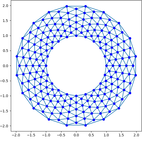
Sample mesh for the annulus

Now we will approximate functions on the annulus by continuous piece-wise linear functions. That is, functions that are linear within each triangle, and continuous across triangles. This seems complicated, but we can simplify this by introducing some basis functions. Enumerate all vertices in the above mesh that lie in the interior of the domain. Then, the \(j^{\rm th}\) basis function is the piece-wise linear function that is equal to 1 on the \(j^{\rm th}\) vertex, and zero over all other vertices. One such function is:

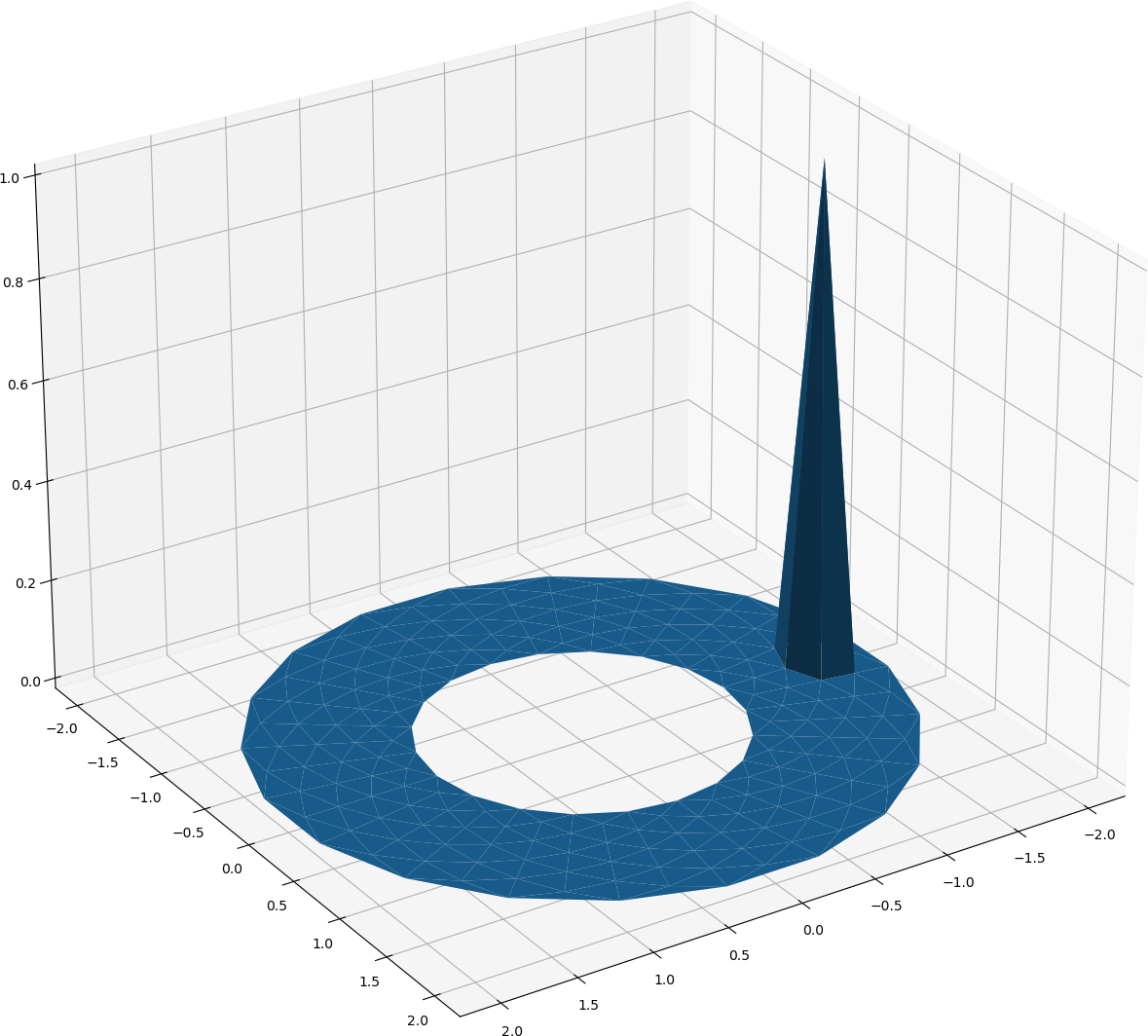
One basis function on the above mesh

Note that due to the solution going to zero on the boundaries (homogeneous Dirichlet boundary conditions) we only need to form basis functions over the interior nodes. Denote each basis function as \(\phi_j(x,y)\)

Ok, what does all of this have to do partial differential equations and the finite element method? We will seek our approximate solution \(\widetilde{u}(x,y)\) as an expansion in these basis functions:

(2)\[\widetilde{u}(x,y) = \sum\limits_{j=0}^{N_{int}} u_j \phi_j(x,y)\]

Now, write the forcing function in the same way, and insert each into the governing PDE to obtain:

(3)\[-\sum\limits_{j=0}^{N_{int}} u_j \nabla^2\phi_j(x,y) = \sum\limits_{j=0}^{N_{int}} f_j \phi_j(x,y)\]

and recall that the boundary conditions are enforced naturally by the choice of basis functions. Do you see a problem here though? Our basis functions are continuous, but we certainly can’t take the Laplacian of them (without getting into some real weird math). Also, this is just one equation, but all of the \(u_j\) coefficients are unknown. How can we find those?

We’ll pull a little trick, multiply the above by another basis function, \(\phi_i(x,y)\), and integrate over the whole domain:

(4)\[\sum\limits_{j=0}^{N_{int}} u_j \int\limits_\Omega\nabla\phi_i\cdot\nabla\phi_j dxdy = \sum\limits_{j=0}^{N_{int}} f_j \int\limits_\Omega\phi_i(x,y)\phi_j(x,y) dxdy\]

where we have used integration by parts on the left hand side. This might not seem any better, but really we are almost all the way through. We will enforce that this equation holds not just for one basis function, but for all \(\phi_i(x,y)\). Do those sums look familiar to you? Of course! These are just the sums for matrix vector multiplication!

In total, all the finite element method boils down to is solving this linear system for the coefficients \(u_j\):

(5)\[\mathbf{K}\mathbf{u} = \mathbf{M}\mathbf{f}\]

where,

(6)\[\begin{split}K_{ij} &= \int\limits_\Omega\nabla\phi_i\cdot\nabla\phi_j dxdy \\ M_{ij} &= \int\limits_\Omega\phi_i(x,y)\phi_j(x,y) dxdy\end{split}\]

These are called the stiffness and mass matrices. The naming comes from the initial development of the finite element method having its roots in structural analysis. These matrices have some special properties, namely that they are both sparse, and symmetric. The stiffness matrix is positive definite as well, which we’ll exploit down below.

The example code

The example code implements the finite element method as described above through 3 header/source file pairs, a main source file, and a couple of supporting Python scripts. The header/source file pairs are:

• SparseMat.h/ SparseMat.c Define a sparse matrix data structure.

  • These are lightly modified from the one given in your homework to support adding entries in a different way. A conjugate gradient routine is also present

• SimpleMesh.h/ SimpleMesh.c Define a simplified mesh data structure that can be initialized from an input file.

• FEMatrices.h/ FEMatrices.c Define routines to fill sparse matrices with respect to a given mesh according to the above definitions

All of these files can be downloaded here: fe_solver.tar.gz

To build the example you can run:

make
python meshGen.py
./FESolver
python plotSol.py

and you should be greeted by a figure. A finer mesh can be used as well:

python meshGen.py 40 80
./FESolver
python plotSol.py

Remark: You still need to fill in the matrix-vector multiplication function in SparseMat.c for this to work. You can directly paste in what you write for the final homework assignment.

The second call above should give the figure:

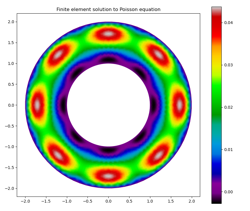
Solution on the mesh with 40 points radially and 80 points azimuthally

The main file:

The main file is really quite simple since most of the heavy lifting happens behind the scenes in the other source files:

/* File: FESolver.c
 * Author: Ian May
 * Purpose: Set up and solve Poisson's equation on a given domain
 */

#include <stdlib.h>
#include <stdio.h>
#include <math.h>

#include "SparseMat.h"
#include "SimpleMesh.h"
#include "FEMatrices.h"

double forcing(double x, double y)
{
  return ((x*x + y*y) - 2.0)*fabs(cos(4.0*atan2(y,x)));
}

int main()
{
  /* Create mesh from file */
  Mesh mesh = NULL;
  CreateMesh("annulus.mesh",&mesh);

  /* Create finite element matrices */
  SparseMat M=NULL, K=NULL;
  CreateMassMatrix(mesh, &M);
  CreateStiffnessMatrix(mesh, &K);
  SparseMatPrintInfo(K,NULL);
  SparseMatSavePattern(K,"stiffnessNNZ.dat");

  /* Evaluate forcing function, create load and solution vectors */
  double forceVec[mesh->nD], loadVec[mesh->nD], solVec[mesh->nD];
  MeshSetForcing(mesh,forceVec,forcing);

  /* Set load vector from forcing vector */
  SparseMatMult(M,forceVec,loadVec);

  /* Solve system using CG */
  SparseMatCG(K,solVec,loadVec,K->n,1.e-8);

  /* Write out solution */
  MeshSaveSol(mesh,solVec,"annulus");
  
  DestroyMesh(&mesh);
  DestroySparseMat(&M);
  DestroySparseMat(&K);
  return 0;
}

There are a few notable things happening here:

• The forcing function is defined here, but passed off to be evaluated elsewhere.

  • This means that we don’t need to think to hard about how to approximate the right hand side in the given function space while thinking about the main program.

• The mesh is created by reading in a file. This means the same code can be used to solve Poisson’s equation on many different domains without any deep changes.

• The mass and stiffness matrices are created by calls to factory functions defined elsewhere. Again, these work for arbitrary (valid) meshes.

• The final linear system is solved using the conjugate gradient method

  • This is beyond the scope of this course, but essentially this solves the above linear system by only using matrix-vector products. Recall from the homework that sparse matrices make this extremely efficient.

• Finally, the solution is saved through another call to the mesh functions.

This gives a nice overview of the method, and what really needs to be done. Next we’ll take a tour of the relevant parts of the other source files.

The SparseMat files:

The sparse matrix implementation used here is only slightly different from the one you’ve seen in your homework. The additions include a function to add entries into existing rows:

/* Specify values and locations for a given row.
 * Must be compatible with corresponding entry in nnz given
 * during call to SparseMatSetNNZ */
void SparseMatAddRow(SparseMat A, int row, int nCols, int *cols, double *vals)
{
  for(int j=0; j<nCols; j++) {
    int idx = -1;
    for(int k=0; k<A->nnz[row]; k++) {
      if(A->cols[row][k] == cols[j]) {
        idx = k;
        break;
      }
    }
    if(idx >= 0) {
      A->rowVals[row][idx] += vals[j];
    } else {
      printf("Warning: Column mismatch in SparseMatAddRow\n");
    }
  }
}

and a few functions to implement the conjugate gradient method mentioned before. Again, the inner workings of this aren’t too important right now, but it is nice to see how simple the implementation really is:

void SparseMatCG(SparseMat A, double x[A->n], double b[A->n], int max_its, double rtol)
{
  printf("Running CG iteration\n");
  double r[A->n], p[A->n], Ap[A->n];
  vecCopy(A->n, b, r);
  vecCopy(A->n, b, p);
  vecZero(A->n,x);
  double rTrnm = vecDot(A->n, r, r);
  double rNorm = sqrt(rTrnm);
  for(int n=0; n<max_its; n++) {
    /* Step length and solution update */
    SparseMatMult(A, p, Ap);
    double pTApn = vecDot(A->n, p, Ap);
    double alpha = rTrnm/pTApn;
    vecAddScaled(A->n, x, alpha, p, x);
    /* Residual update and convergence check */
    vecAddScaled(A->n, r, -alpha, Ap, r);
    double rTrn = vecDot(A->n, r, r);
    if(sqrt(rTrn)/rNorm < rtol) {
      printf(" CG iteration converged, iterations: %d, reltol: %e\n",n+1,sqrt(rTrn)/rNorm);
      break;
    } else if(n==max_its-1) {
      printf(" CG iteration failed, iterations: %d, reltol: %e\n",n+1,sqrt(rTrn)/rNorm);
    }
    /* Update search direction and dot prods */
    vecAddScaled(A->n, r, rTrn/rTrnm, p, p);
    rTrnm = rTrn;
    }
  }

Finally, a function that writes out the sparsity pattern has been added to help visualize what these things actually look like:

void SparseMatSavePattern(SparseMat A, const char *fname)
{
  /* Open file and write non-zero positions as x-y coords */
  FILE *fp = fopen(fname,"w");
  for(int i=0; i<A->m; i++) {
    for(int j=0; j<A->nnz[i]; j++) {
      fprintf(fp,"%d %d\n",A->m-i,A->cols[i][j]);
    }
  }
  fclose(fp);
}

The mesh files:

The mesh data structure is defined as:

typedef struct _p_Mesh *Mesh;

typedef struct {
  int v0, v1, v2; /* Indices of vertices */
} Face;

typedef struct {
  double x, y; /* Coords of vertex */
  bool bdy;    /* Is vertex on the boundary */
} Vertex;

struct _p_Mesh {
  int nV, nD, nF;         /* Number of faces, vertices, DOFs */
  int *idx2dof, *dof2idx; /* Maps between vertex idx and dof index */
  Face *faces;            /* Array of faces */
  Vertex *verts;          /* Array of vertices */
};

That is, the mesh stores:

• An array of the coordinates and type of each vertex

• An array of faces that consist of three integers which index back into the vertex array

• Arrays that convert between the indexing of the vertices including and not including the boundaries

All of these fields are read in from a file by the function:

void CreateMesh(const char *meshFile, Mesh *a_mesh)
{
  /* Open mesh file */
  FILE *fp = fopen(meshFile,"r");
  char line[MAX_LINE_LENGTH];

  /* Allocate mesh struct */
  Mesh mesh = malloc(sizeof(struct _p_Mesh));
  /* discard first line, then read in counts */
  fgets(line,MAX_LINE_LENGTH,fp);
  fscanf(fp,"%d %d %d\n",&mesh->nV,&mesh->nD,&mesh->nF);
  mesh->verts = malloc(mesh->nV*sizeof(*mesh->verts));
  mesh->faces = malloc(mesh->nF*sizeof(*mesh->faces));
  mesh->idx2dof = malloc(mesh->nV*sizeof(*mesh->idx2dof));
  mesh->dof2idx = malloc(mesh->nD*sizeof(*mesh->dof2idx));

  /* Discard line and read in vertices */
  fgets(line,MAX_LINE_LENGTH,fp);
  int dCtr=0, vType;
  for(int n=0; n<mesh->nV; n++) {
    fscanf(fp,"%lf %lf %d\n",&mesh->verts[n].x,&mesh->verts[n].y,&vType);
    mesh->verts[n].bdy = (vType == 0);
    if(mesh->verts[n].bdy) {
      mesh->idx2dof[n] = -1;
    } else {
      mesh->idx2dof[n] = dCtr;
      mesh->dof2idx[dCtr] = n;
      dCtr++;
    }
  }

  /* Discard line and read in faces */
  fgets(line,MAX_LINE_LENGTH,fp);
  for(int n=0; n<mesh->nF; n++) {
    fscanf(fp,"%d %d %d\n",&mesh->faces[n].v0,&mesh->faces[n].v1,&mesh->faces[n].v2);
  }

  fclose(fp);

  *a_mesh = mesh;
}

It might look a little busy, but you should recognize everything happening here from the section on file input/output. Notice that fgets is occasionally used to discard lines in the mesh file that are just there for us humans to read.

The FE matrix files:

The file FEMatrices.c encodes most of the math going on in this example code. Really, the stiffness and mass matrices can be constructed using nothing more than what you learned, or will learn, in multi-variable calculus. Actually, it’s a bit simpler since the domains are always triangles, and the functions to be integrated are quadratic at worst.

Let’s just extract one section from the constructor for the mass matrix:

/* Loop over faces and add in each contribution */
for(int nF=0; nF<mesh->nF; nF++) {
  /* Get indices and dof numbers */
  int v0=mesh->faces[nF].v0, v1=mesh->faces[nF].v1, v2=mesh->faces[nF].v2;
  int d0=mesh->idx2dof[v0], d1=mesh->idx2dof[v1], d2=mesh->idx2dof[v2];
  /* Find Jacobian to transform to ref. element */
  double J = (mesh->verts[v1].x-mesh->verts[v0].x)*(mesh->verts[v2].y-mesh->verts[v0].y);
  J -= (mesh->verts[v2].x-mesh->verts[v0].x)*(mesh->verts[v1].y-mesh->verts[v0].y);
  J = fabs(J);
  /* Form all entries */
  double vals[] = {J/12., J/24., J/24.};
  /* Form entries for d0 */
  if(d0 >= 0) {
    int nCols = 1;
    int cols[] = {d0,-1,-1};
    if(d1 >= 0) {
      cols[nCols] = d1;
      nCols++;
    }
    if(d2 >= 0) {
      cols[nCols] = d2;
      nCols++;
    }
    SparseMatAddRow(M,d0,nCols,cols,vals);
  }
  /* Do the same for d1 and d2 */
  /* ... */
}

Note that this is really quite similar to what you are doing in your homework, just now we are potentially adding to entries that are already present in the matrix. Of course, finding the correct column indices is also a little bit more complicated than the tri-diagonal matrix seen in the assignment.

Wrapping up

Try experimenting with different mesh refinements and forcing functions. The python helper script meshGen.py creates the mesh files. The calling convention is

python meshGen.py <numRad> <numTheta>

where the two command line arguments are the number of points in the radial and azimuthal directions respectively. The total number of unknowns that the finite element code has to solve for will be the product of these numbers (well, slightly less). I can report that even up to 200 radial points and 400 azimuthal points will give a solution fairly quickly, though the python plotting routines will start to struggle.

You could even try writing your own mesh file. Try running the generator with a really small number of points, like

python meshGen.py 5 10

then look at the file annulus.mesh to get a feel for what should be present. Note that the third column in the vertices section denotes whether a vertex is on the boundary or not. These don’t need to go in order, it just happened to be easier to write all of the boundary points first in this case.

Enjoy!